[산업공학(IE)] 6편(완결): 워크샘플링과 여유시간 — 현장 전체를 순간포착으로 진단하기[Industrial Engineering (IE)] Part 6 (Final): Work Sampling and Allowances — Diagnosing the Whole Floor by Snapshot

5편까지는 스톱워치로 한 작업자를 처음부터 끝까지 관측하는 방식을 다뤘습니다. 이번 마지막 편은 접근이 완전히 다릅니다. 현장 전체를 정해진 시각에 "순간 스냅샷"처럼 찍어서, 통계적으로 가동 상태를 추정하는 워크샘플링(Work Sampling)입니다. 여기에 표준시간의 마지막 퍼즐 조각인 레이팅과 여유시간까지 정리하며 IE 시리즈를 마무리합니다.

워크샘플링이란

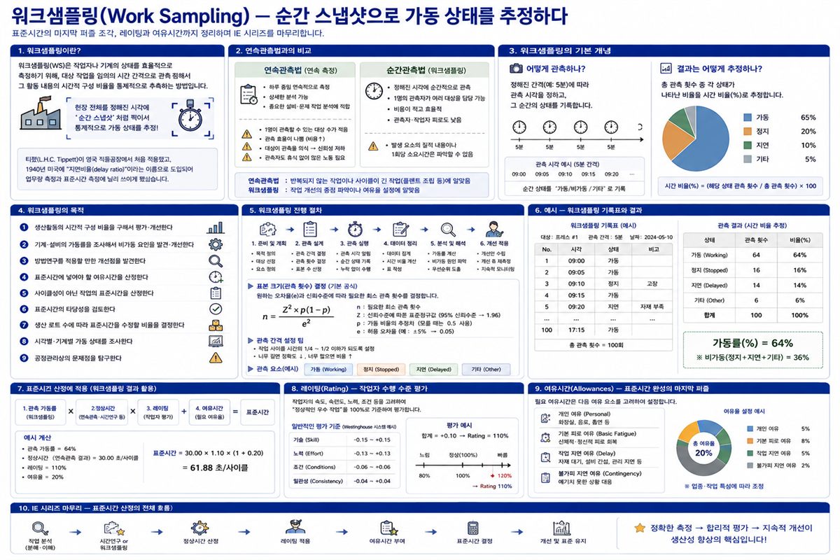
워크샘플링(WS)은 작업자나 기계의 상태를 효율적으로 측정하기 위해, 대상 작업을 임의의 시간 간격으로 관측해서 그 활동 내용의 시간적 구성 비율을 통계적으로 추측하는 방법입니다. 티펫(L.H.C. Tippett)이 영국 직물공장에서 처음 적용했고, 1940년 미국에 "지연비율(delay ratio)"이라는 이름으로 도입되어 업무량 측정과 표준시간 측정에 널리 쓰이게 됐습니다.

연속관측법과의 비교

가동 분석에는 크게 두 갈래가 있습니다.

구분	연속관측법	순간관측법(워크샘플링)
관측 방식	하루 종일 연속 측정	정해진 시각에 순간 관측
1인 담당 대상	적음	많음 (비용 절감)
관측자·작업자 피로	높음	낮음
결과 신뢰성	의식 효과로 낮아질 수 있음	순간 관측이라 왜곡 적음
발생 요소의 질·소요시간	파악 가능	파악 불가
적합 용도	반복 없는 작업, 긴 사이클(플랜트 등)	작업개선 과제 파악, 여유율 설정

워크샘플링의 목적

• 생산활동의 시간적 구성 비율을 구해서 평가·개선한다
• 기계·설비의 가동률을 조사해서 비가동 요인을 발견·개선한다
• 방법연구를 적용할 만한 개선점을 발견한다
• 표준시간에 넣어야 할 여유시간을 산정한다
• 사이클성이 아닌 작업의 표준시간을 산정한다
• 표준시간의 타당성을 검토한다
• 생산 로트 수에 따라 표준시간을 수정할 비율을 결정한다
• 시각별·기계별 가동 상태를 조사한다
• 공정관리상의 문제점을 탐구한다

특징

측정 효율이 좋고 경제적입니다(순간관측이라 1명이 여러 대상 담당 가능). 순간관측이라 작업자의 의식이 적어 왜곡이 적은 정확한 결과를 얻습니다. 훈련도 거의 필요 없고, 랜덤 관측을 하면 관측오차를 관측 횟수로 산출할 수 있어 결과의 정도가 보증됩니다.

워크샘플링 실시 12단계

1단계: 목적을 정한다. 목적은 크게 두 가지 — 생산 저해 요인을 파악해서 작업개선 과제를 설정하거나, 표준시간 설정을 위한 여유율을 구하는 것. 목적에 따라 관측 세부 항목이 크게 달라집니다.

2단계: 관계자의 이해와 협력을 얻는다. 현장 관계자에게 목적과 방법을 충실히 설명해야 소기의 목적을 달성할 수 있습니다.

3단계: 관측 대상의 범위를 정한다. 감독자, 준비 작업자, 운반 작업자 등 목적에 맞게 범위를 정합니다.

4단계: 관측 대상을 층별한다. 층별을 너무 세밀하게 하면 관측 횟수가 많이 필요해서 오차가 커집니다. 보통 작업자는 현장별·직종별·성별·경험연수별로, 기계는 현장별·기종별·능력별로 층별합니다.

5단계: 관측 항목을 정한다. 가장 중요한 단계입니다. 관측자가 여럿일 때는 해석 기준을 반드시 통일해야 합니다.

• 관측 전에 현장을 충분히 관찰해서 발생 요소를 파악해둔다
• 발생 요소는 구체적으로 정한다 — "준비작업", "기계조정" 같은 추상적 표현은 피한다
• "협의와 잡담", "대기와 손놓기"처럼 관측자의 주관적 판단에 좌우되는 구분은 피한다
• 기계 현장은 "기계가동 중"/"기계정지 중"으로, 라인 생산은 "라인가동 중"/"라인정지 중"으로 나눠 관측한다
• 관측 항목란 끝에는 반드시 "부재" 항목을 둔다

6단계: 관측 수를 정한다. 관측수는 관측 대상수 × 관측 횟수로 구하며, 관측수가 커질수록 오차는 작아집니다.

관측 목적	발생률(p)	절대오차(e)	상대오차	관측수(n)
가동 저해 요인 조사	15%	1.5~2.5%	10~17%	800~2,200
여유율의 결정	20%	1.2~1.8%	6~9%	2,000~5,000
사이클당 실질 작업시간 결정	70%	1.4~2.1%	2~3%	2,000~5,000

관측 횟수 계산식(신뢰도 95%, Z=2):

N = Z² · p(1-p) / e²
(e: 절대오차, Z: 신뢰도 계수, p: 발생률)

하루 관측 횟수는 10회 이상으로 합니다. 관측 기간은 사이클이 짧으면 1주일 정도, 비사이클 작업이면 더 길게 잡되 2주일 이상 연속 관측은 비효율적입니다.

7단계: 관측 시각을 정한다. 랜덤 샘플링법과 등시간 간격법 중, 데이터 편차를 피하기 위해 랜덤 샘플링을 권장합니다.

8단계: 관측 경로와 지점을 정한다. 왔다갔다하지 않도록 효율적인 경로를 정합니다. 관측 지점에 도착하기 전까지는 오히려 관측 대상에서 시선을 떼고, 지점에 도착했을 때 대상을 보는 게 절도 있는 관측입니다.

9단계: 관측 용지를 준비한다. 관측 항목을 순서대로 적어두고, 한 장에 다 채워지도록 설계합니다. 항목이 많으면 5칸마다 붉은 줄을 그어 기입 오류를 방지합니다.

10단계: 예비 관측을 한다. 관측 항목·경로·지점이 적절한지 확인하기 위해 5회 정도 미리 해봅니다.

11단계: 관측을 실시한다. 작업자에게 불쾌감을 주지 않는 절도 있는 태도로 관측하고, 순간적으로 판별하기 어려우면 뒤이어지는 동작으로 판단합니다. 원칙적으로 한 사람씩 관측합니다. 작업자가 관측을 의식해서 부자연스러운 행동(괜히 부품을 들여다보거나 기름걸레로 작업대를 훔치는 등)을 하는 경우도 있습니다.

12단계: 관측 자료를 개선 계획이나 표준시간에 활용한다.

실전 예시: 랜덤 시각 설정

작업자 15명의 조립 현장을 일일 20회씩 4일간 관측한다고 해봅시다. 취업시간은 8:30~17:00, 점심시간은 12:00부터 45분, 10:00와 15:00부터 10분씩 휴식이 있습니다. 랜덤시각표에서 한 열을 골라 왼쪽 숫자 순서로 시각을 매핑합니다(예: 0.01=8시 1분). 도중 점심시간에 해당하면 제외하고, 오전·오후 10분 휴식 시간대에 해당하는 관측 시각은 그대로 채택합니다 — 이때는 15명을 동시에 관측하는 게 아니라, 현장 출입구를 향해 관측하러 "출발하는" 시각을 의미하기 때문입니다. 휴식 시작·종료를 알리는 벨 소리를 듣고 관측하면 휴식 전후의 작업 상태까지 파악할 수 있습니다.

워크샘플링의 종류

• 퍼포먼스 워크샘플링: 관측과 동시에 레이팅까지 하는 방법. 사이클이 매우 길거나 그룹 작업처럼 전형적인 시간측정으로 표준시간을 정하기 어려울 때 씀
• 체계적 워크샘플링: 균등한 시간 간격으로 관측 시각을 만드는 방법
• 층별 샘플링: 층별로 구분해서 연구한 뒤 가중평균치를 구하는 방법

워크샘플링 결과 분석

목적이 "작업개선"이냐 "여유율 설정"이냐에 따라 절차가 갈립니다.

작업개선의 경우: 각 관측항목의 구성비율 계산 → 여유·기타 요소 항목별 구성비율 계산 → 업무구분별 구성비율 계산 → 전체 가동상황을 원그래프·띠그래프로 시각화 → 구성비율이 큰 항목부터 파레토 분석도를 만들어 가동 저해 요인을 찾는다.

여유율 설정의 경우: 표준시간에 넣을 필요 없는 항목(수정, 대기 등) 제외 → 정기적인 조회·휴식 시간을 하루 가동시간에서 미리 뺀다 → 작업여유·현장여유 각 항목의 관측도수 합계가 주체작업 도수의 몇 %인지 계산하면 그게 곧 여유율입니다.

주의할 점은, 인적여유·피로여유는 워크샘플링으로는 설정할 수 없다는 것입니다. 이 부분은 학자·연구자가 제시하는 여러 여유율을 참고해서 각 기업의 방침에 따라 설정합니다.

개선안 검토

워크샘플링은 공정분석과 마찬가지로, 개별 공정 분석에 앞서 현장 전체의 가동 상태를 파악하는 게 주목적입니다. 여기서 나온 문제점은 다시 연합작업분석·시간연구 같은 다른 IE 기법으로 더 깊이 파고듭니다.

분석 결과	문제 영역	요인 분석 기법
운반·보행·부재가 많다	레이아웃, 라인밸런스, 기계 점유대수	공정분석, 운반분석, 라인밸런싱, 연합작업분석
대기가 많다	재료·부품 조달, 설비	유동수분석(재고관리), 설비관리
협의가 많다	작업지시·지도	공정관리, 교육훈련
손놓기·잡담이 많다	현장 규율	관리감독자의 역할

레이팅: 관측시간을 정미시간으로 바꾸기

레이팅은 관측시간을 정미시간으로 변환하기 위해, 관측자가 훈련으로 구축한 표준 페이스와 관측 대상의 작업 페이스를 비교해서 평가하는 것입니다.

레이팅의 종류

• 속도평가법(스피드 레이팅): 작업 속도만으로 평가
• 노력평가법: 작업의 곤란성·숙련도·노력도·작업조건을 종합 고려
• 합성평가법 / 객관적평가법: 2차 조정계수를 이용. Tn = Po(1+S) (Tn: 정미시간, Po: 1차 속도평가계수, S: 2차 조정계수)
• 평준화법(웨스팅하우스법, Leveling): 숙련도·노력도·작업조건·작업의 일치성을 종합 고려

레이팅의 경향(오류)

• 극단적 레이팅: 늦은 작업은 더 늦게, 빠른 작업은 더 빠르게 판정 — 대비 효과 때문
• 보수적 레이팅: 늦은 작업은 빠르게, 빠른 작업은 늦게 평가 — 훈련 초기에 자주 나타남
• 후한 레이팅 / 엄한 레이팅: 전반적으로 관대하거나 박하게 평가하는 경향

표준시간: 다시 정리하면

표준시간이란 작업시간에 영향을 미치는 작업방법·조건·작업자·속도·여유의 표준적인 상태를 가정해서 구한 조건부 시간이며, 기준치 또는 목표치로서의 성격을 갖습니다.

풀어서 말하면: 그 작업에 적성을 갖고 숙련된 작업자가, 특정 작업환경 아래에서, 필요한 여유를 가지고, 정해진 작업방법·조건·설비로, 표준적인 노력을 통해 일정한 양과 질의 작업을 완성하는 데 필요한 시간입니다.

표준시간의 용도

목적	활용 사례
계획	생산계획·일정계획, 원가견적과 판매가격 설정, 공정 밸런싱, 설비·요원 산정, 1일 작업량 결정
관리	감독지도와 목표설정, 능률급 설정, 예산통제와 원가관리, 작업훈련
평가	작업방법의 비교·개선·선택, 생산설비와 배치 설계 비교, 직무평가, 생산성 측정

표준시간의 구성

표준시간 = 주작업시간 + 준비작업시간
         = 정미시간 + 여유시간

여유시간, 제대로 파고들기

여유시간의 분류

여유는 두 축으로 분류합니다.

항목에 따른 분류: 일반여유(인적여유, 불가피지연여유, 피로여유) / 특수여유(기계간섭여유, 조여유, 소로트여유, 기타)

적용 대상에 따른 분류: 작업사이클 전체에 적용되는 여유 / 기계 가공시간에만 적용되는 여유 / 작업자 시간에만 적용되는 여유

일반여유는 어떤 작업이든 감안해주는 여유로, 영어 앞글자를 따서 PDF여유(Personal, Delay, Fatigue)라고도 부릅니다.

여유율의 두 가지 표시법: 외경법(A) vs 내경법(B)

여유율 A (정미시간 대비, 외경법)

여유율 A(%) = 일반여유시간 / 정미시간 × 100
표준시간 = 정미시간 × (1 + 여유율 A)

ILO의 여유율표도 이 방식을 따릅니다.

여유율 B (근로시간 대비, 내경법)

여유율 B(%) = 일반여유시간 / 근무시간 × 100
표준시간 = 정미시간 × [100 / (100 - 여유율 B)]

실전 계산 예시: 두 방식을 헷갈리면 벌어지는 일

평균관측시간 0.8분, 레이팅계수 110%, 여유시간이 하루 8시간 근무 중 24분이라고 해봅시다.

여유율 = 24/480 × 100 = 5%. 이걸 외경법 공식에 잘못 대입하면: 표준시간 = (0.8)(1.1)(1+0.05) = 0.924분.

하지만 이 여유율은 근무시간(480분) 대비로 정의된 값(여유율 B)이므로 내경법 공식을 써야 합니다: 표준시간 = (0.8)(1.1) × [1/(1-0.05)] = 0.9263분.

검증: 정미시간 0.88분이므로 여유시간 24분을 뺀 456분 동안 456÷0.88 = 518.18개 생산 → 8시간(480분) 기준 480÷518.18 = 0.9263분/개. 내경법 결과와 정확히 일치합니다.

교훈: 경영진이 "여유율 10%"라고 통보했을 때, 관측자는 이게 정미시간 기준(외경법 A)인지 근무시간 기준(내경법 B)인지 반드시 확인해야 합니다.

일반여유 상세

① 인적여유 (Personal Allowance)

물마시기, 화장실, 땀닦기, 재채기 등 생리적 욕구로 인한 지연을 보상합니다. Lazarus가 235개 공장을 조사한 결과 평균 5.6%였고, 목재벌채·가공산업은 10%, 금속소재산업은 7.6%로 업종마다 크게 달랐습니다. ILO는 남자 5%, 여자 7%로 정했지만, 이게 과학적으로 확실한 근거를 가진 수치는 아니라는 점도 함께 지적됩니다.

② 피로여유 (Fatigue Allowance)

작업 수행에 따른 정신적·육체적 피로를 회복하기 위한 여유입니다. 개인차가 커서 객관적 측정이 어렵다는 게 현재도 논란거리입니다. Eugene Brey는 이런 피로계수(F) 공식을 제안했습니다.

F = (T - t) × 100 / T
(T: 연속작업 중 마지막 사이클 시간, t: 연속작업 중 첫 번째 사이클 시간)

피로 측정법은 크게 세 유형으로 나뉩니다.

• 물리적 검사: Dynamometer 등으로 근육 운동 능력의 변화 측정
• 화학적 검사: 피로가 인체 분비물이나 혈액 성분에 미치는 영향 조사
• 생리학적 검사: 맥박·혈압·호흡수·산소흡입량·탄산가스 생성량·에너지소모량 등 측정. 최근 연구는 주로 이 쪽에 집중

RMR(에너지대사율)을 이용한 피로여유율 산정도 있습니다.

RMR = [작업시대사량(C) - 안정시대사량(C1)] / 기초대사량(Co)

RMR값이 높을수록 노동 강도가 세다고 봅니다(0~0.9는 아주 가벼움, 7.0 이상은 아주 강함). 피로여유율은 정신적 노력(Fa), 육체적 노력(Fb), 단조감(Fc), 유휴시간 회복계수(L)를 조합해서 산정합니다: F = (Fa+Fb)L+Fc.

③ 불가피지연 여유 (Unavoidable Delay)

작업자 능력 밖의 사유로 지연되는 부분을 보상합니다.

• 조장·직장 등에 의한 지연 (품질·계획 관련 논의)
• 재료 품질 불균일에 의한 지연
• 기계·공구 보전 및 조정에 의한 지연 (공구 파손, 설비 조정, 오일 주입 등)
• 작업 완료 전 간단한 청소 (단, 청소가 독립 작업으로 표준시간이 따로 있으면 제외)

지연 여유를 설정하는 대표적 기법이 바로 워크샘플링과, 장시간 지속 관찰하며 지연 사유·시간을 매번 기록하는 가동연구입니다. 가동연구의 단점은 관측자·작업자 모두 장시간 관측에 지치고, 샘플 수가 적어 오차가 커질 수 있다는 점입니다.

특수여유 상세

① 기계간섭여유

작업자 1명이 동일 기계를 여러 대 담당할 때, 한 기계를 조작하는 동안 다른 기계는 멈춰 있는 현상 때문에 생산량이 줄어드는 걸 보상합니다. Wright는 기계 대수가 7대 이상일 때 이런 공식을 제안했습니다.

I = 50 × [√((1+R-N)² + 2N) - (1+R-N)]
(N: 담당 기계대수, R: 평균기계가동시간/평균손취급시간, I: 평균손취급시간 대비 기계간섭율%)

계산 예시: 섬유공장에서 작업자 1명이 Spindle 60대 담당, 제품 1개당 평균기계시간 150분, 평균 손취급시간 3분이라면:

• R = 150/3 = 50, N = 60
• I ≈ 1,160%
• 기계간섭시간 = (11.6)(3분) = 34.8분
• 표준시간(60대 기준) = 150 + 3 + 34.8 = 187.8분
• 제품 1개당 표준시간 = 187.8 / 60 = 3.13분

② 조여유

컨베이어 작업처럼 조를 이루어 작업할 때, 서로 보조를 맞추느라 생기는 불가피한 지연을 보상합니다.

③ 소로트여유

작업자의 능률은 어느 정도 워밍업이 되어야 오릅니다. 능률이 100%에 도달하기까지 필요한 최소 로트 크기에 못 미치는 소량만 생산할 때는, 제품 1개당 표준시간을 조금 늘려주기도 합니다.

④ 기타여유 (장사이클여유, 기계여유)

사이클이 비교적 길어 작업 내용의 변동 가능성을 감안하는 장사이클여유가 있고, 장려급 제도 하에서 작업자 요소작업과 기계 요소작업의 균형을 맞추기 위한 기계여유도 있습니다. 예를 들어 기계요소작업이 2분, 작업자요소작업 표준시간이 1분인 사이클에서 작업자가 125% 수준으로 열심히 일해도 전체로는 107%밖에 달성하지 못하는 구조라면, 다른 작업자와 형평을 맞추기 위해 기계요소작업에 인위적으로 여유를 더해줍니다.

⑤ 장려여유

임금 지급과 관련된 정책적 여유로, 평균적인 작업자가 기본급 대비 몇 %의 할증금을 받을 수 있는지를 결정합니다.

---

시리즈를 마무리하며

여섯 편에 걸쳐 IE(산업공학) 교재 한 권을 통째로 훑어봤습니다. 다시 정리하면 이런 흐름이었습니다.

1. 1편: IE의 정의, 테일러·길브레스의 역사, 호손 실험 — "왜 이런 학문이 생겼는가"
2. 2편: 방법연구와 공정분석 — "공정 전체를 어떻게 도표로 그려서 낭비를 찾는가"
3. 3편: 작업분석과 표준자료법 — "사람과 기계를 어떻게 배치해야 경제적인가"
4. 4편: 동작연구와 동작경제의 원칙 — "손끝 하나의 움직임까지 어떻게 최적화하는가"
5. 5편: 스톱워치 시간연구 실무 — "표준시간을 어떻게 정확하고 공정하게 재는가"
6. 6편: 워크샘플링과 여유시간 — "현장 전체를 어떻게 통계적으로 진단하고, 인간적인 여유를 어떻게 합리적으로 반영하는가"

큰 그림에서 보면 이 학문은 결국 두 가지를 동시에 추구합니다. 테일러가 대표하는 정량적·과학적 측정과, 호손 실험이 보여준 인간에 대한 이해입니다. 표준시간 하나를 정하는 데도 스톱워치의 정밀함과 피로·여유에 대한 배려가 함께 들어가야 한다는 걸, 이번 시리즈를 통해 확인할 수 있었습니다.

Parts 1–5 dealt with following a single worker from start to finish with a stopwatch. This final part takes a completely different approach: snapping a statistical "photograph" of the entire floor at predetermined random moments to estimate activity composition — Work Sampling (WS). This part also completes the standard-time picture by covering performance rating and allowance time in full detail.

What Is Work Sampling?

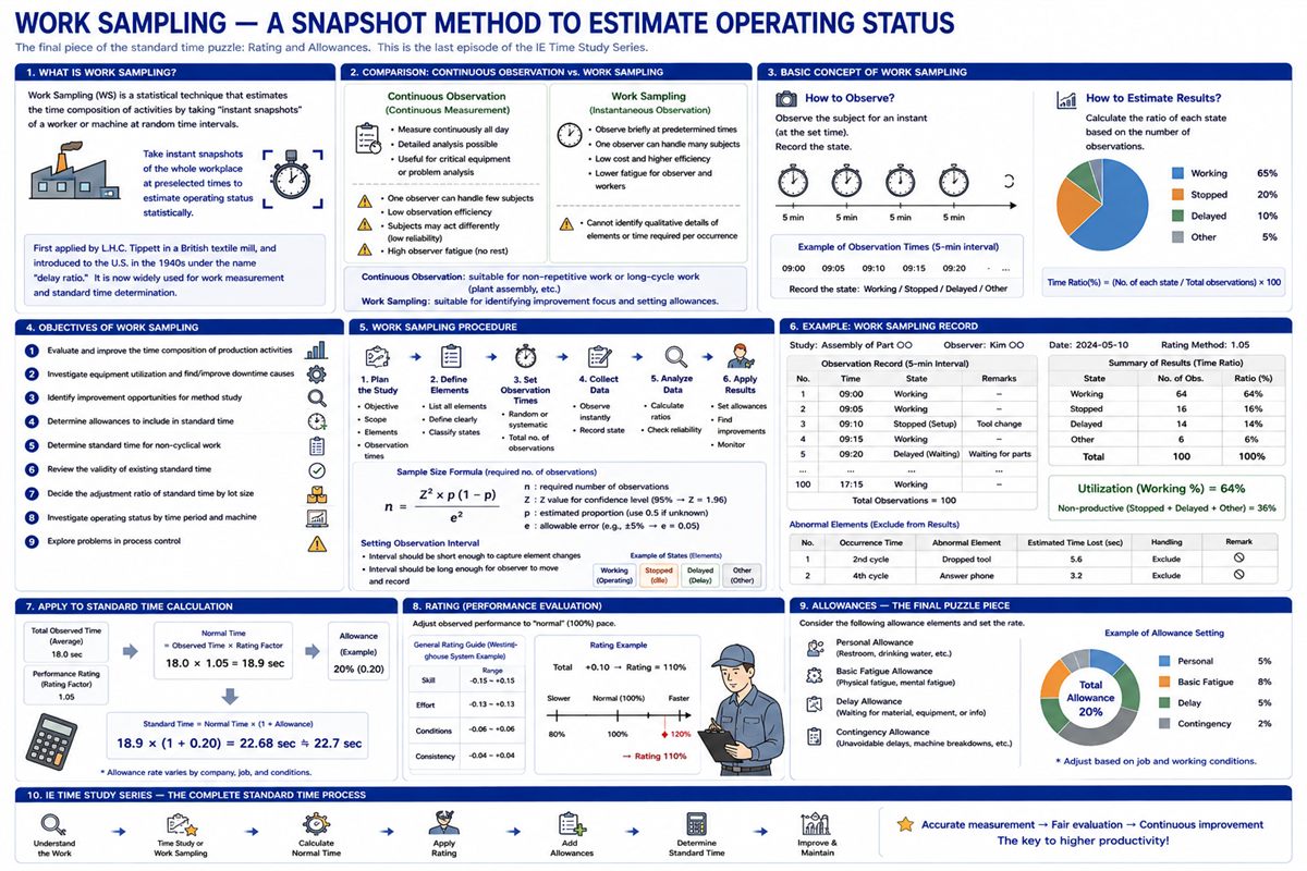
Work sampling is a method for efficiently measuring the state of workers or machines by observing them at random time intervals and statistically inferring the proportion of time spent in each activity. L.H.C. Tippett first applied it in British textile mills; the technique reached the United States in 1940 under the name "delay ratio study" and subsequently spread to work measurement and standard-time setting across industries.

Work Sampling vs. Continuous Observation

Two broad approaches exist for activity analysis:

Aspect	Continuous observation	Work sampling (instantaneous)
Observation mode	All-day continuous recording	Instantaneous readings at set times
Subjects per observer	Few	Many (lower cost)
Observer / worker fatigue	High	Low
Result reliability	May drop if worker becomes self-conscious	Instant reading leaves little time for artificial behavior
Event content / duration	Obtainable	Not obtainable
Best applications	Non-repetitive or long-cycle operations (plant assembly, etc.)	Identifying improvement priorities; setting allowances

Objectives of Work Sampling

• Determine the time composition of production activities for evaluation and improvement
• Measure machine and equipment utilization; identify and reduce idle time causes
• Discover opportunities for methods research
• Determine allowance time for inclusion in standard time
• Set standard time for non-cyclic operations
• Verify the validity of existing standard times
• Determine adjustment ratios for standard time by production lot size
• Study utilization by time of day or by machine
• Diagnose production control problems

Key Characteristics

Work sampling is economical and efficient — one observer can cover many subjects with instantaneous readings. Because observations are momentary, workers have little time to alter their behavior, producing more accurate results. Minimal training is required. With random observation timing, the measurement error can be calculated from the number of observations, giving a statistically guaranteed confidence level.

The 12-Step Work Sampling Procedure

Step 1: Define the objective. The two primary goals are: (a) identifying productivity bottlenecks to set improvement priorities, or (b) determining allowances for standard time setting. The objective drives the choice of observation categories.

Step 2: Secure understanding and cooperation. Explain the purpose and method clearly to everyone on the floor. Without this, results may be compromised.

Step 3: Define the scope of observation. Decide who or what to observe — supervisors, setup workers, material handlers — based on the objective.

Step 4: Stratify the subjects. Over-stratification requires more observations and increases error. Workers are typically stratified by work area, job type, gender, and experience; machines by area, type, and capacity.

Step 5: Define observation categories. This is the most critical step. When multiple observers are used, category definitions must be unified.

• Observe the floor in advance to identify what events actually occur
• Define categories specifically — avoid vague labels like "preparation" or "machine adjustment"
• Avoid distinctions that depend on the observer's subjective judgment, such as "discussion vs. chatting" or "waiting vs. idle"
• For machine shops: use "machine running" / "machine stopped"; for line production: "line running" / "line stopped"
• Always include an "absent" category at the end of the observation sheet

Step 6: Determine the number of observations. Total observations = number of subjects × number of readings. Larger samples reduce error. The required observation count (at 95% confidence, Z = 2):

N = Z² · p(1-p) / e²
(e = absolute error, Z = confidence factor, p = occurrence rate)

Objective	p	Absolute error (e)	Relative error	Required N
Identify idle-time causes	15%	1.5–2.5%	10–17%	800–2,200
Determine allowance rates	20%	1.2–1.8%	6–9%	2,000–5,000
Determine productive time per cycle	70%	1.4–2.1%	2–3%	2,000–5,000

Take at least 10 readings per day. Study duration: roughly one week for short-cycle operations; longer for irregular or long-cycle work. Continuous studies beyond two weeks are generally impractical.

Step 7: Set observation times. Random sampling is generally preferred over equal-interval timing to avoid systematic bias.

Step 8: Plan the observation route and points. Design an efficient path that avoids backtracking. Keep your eyes away from the subjects until you arrive at each observation point — look only at the moment of arrival for disciplined, unbiased readings.

Step 9: Prepare observation sheets. List categories in order; design each sheet to hold a full day's data. Use tally marks, and draw a red line every five marks to prevent counting errors.

Step 10: Conduct a pilot study. Run five or so trial observations to verify that categories, route, and points are appropriate before beginning in earnest.

Step 11: Conduct the study. Approach each observation point with a neutral, non-threatening demeanor. If an activity is ambiguous at first glance, let the next motion clarify it. Observe one person at a time — recording multiple workers in sequence and checking them all at once invites mistakes. Workers sometimes perform artificially natural-looking behavior when they notice the observer (pointlessly examining a part, wiping the workbench with an oily rag). An observer unfamiliar with the operation may need to record such moments as "idle" or "waiting" based on contextual judgment.

Step 12: Apply the results to improvement plans or standard time setting.

Example: Setting Random Observation Times

Suppose you are studying 15 assembly workers over 4 days with 20 observations per day. The shift runs 8:30–17:00 with a 45-minute lunch from 12:00 and two 10-minute breaks at 10:00 and 15:00. Select a column from a random-number table and map values to clock times (e.g., 0.01 = 8:01 a.m.). Drop any times that fall during lunch; keep times that fall during the short breaks — these represent the moment the observer departs toward the floor, not the moment all 15 workers are observed simultaneously. Listening for the break bell and observing just as it rings captures before-and-after break behavior in one pass.

Types of Work Sampling

• Performance work sampling: Rating is performed simultaneously with each observation. Used when standard timing methods cannot easily handle very long cycles or group operations.
• Systematic work sampling: Observation times are spaced at equal intervals.
• Stratified sampling: Subjects are divided into strata, studied separately, and results combined by weighted average.

Analyzing Work Sampling Results

For improvement purposes: calculate the percentage of observations for each category → compute sub-percentages for idle and miscellaneous categories → summarize by work type → visualize in pie or bar charts → rank categories by frequency in a Pareto chart to identify the dominant causes of lost productivity.

For allowance setting: exclude categories that should not appear in standard time (rework, avoidable waiting, etc.) → subtract scheduled breaks and meetings from total available time → the percentage of observations in work-allowance and shop-allowance categories relative to productive-work observations directly gives the allowance rate.

Important: personal allowance and fatigue allowance cannot be set by work sampling. These must be determined from research literature and company policy.

Directing Improvement Efforts

Like process analysis, work sampling is primarily a diagnostic tool for the floor as a whole. Problems surfaced here are then investigated in depth with other IE techniques (combined operation analysis, time study, etc.).

Finding	Problem area	Analytical method
High transport / walking / absence	Layout, line balance, machine assignment	Process analysis, transport analysis, line balancing, combined operation analysis
High waiting	Material / component supply, equipment	Flow-count analysis (inventory control), equipment management
High consultation	Work instruction and supervision	Production control, training
High idle / chatting	Floor discipline	Supervisory role

Rating: Converting Observed Time to Normal Time

Rating is the process of comparing the pace of the observed worker to the analyst's internalized standard pace — developed through training — to derive a rating factor that converts observed time to normal (100%) time.

Types of Rating

• Speed rating: evaluates pace only
• Effort rating: accounts for difficulty, skill, effort, and working conditions
• Synthetic / objective rating: uses a secondary adjustment factor: Tn = Po(1+S), where Tn is normal time, Po is the primary speed factor, and S is the secondary adjustment
• Leveling (Westinghouse method): evaluates skill, effort, conditions, and consistency together

Common Rating Errors

• Extreme rating: slow work rated even slower, fast work rated even faster — a contrast effect
• Conservative rating: slow work rated faster, fast work rated slower — common early in training
• Lenient / strict rating: systematic tendency to rate everyone too high or too low

Standard Time: Final Summary

Standard time is a conditional time derived by assuming standard states for the work method, conditions, worker, pace, and allowances — it serves as a reference value or target.

In plain terms: the time required for a skilled worker suited to the job, working under specific conditions with necessary allowances, using the specified method and equipment, and applying standard effort, to complete a unit of work meeting the defined quality and quantity requirements.

Uses of Standard Time

Purpose	Applications
Planning	Production and scheduling plans, cost estimates and pricing, process balancing, equipment and staffing requirements, daily output targets
Control	Supervisory targets, incentive pay design, budget control and cost management, operator training
Evaluation	Comparing and selecting work methods, evaluating plant layout options, job evaluation, productivity measurement

Structure of Standard Time

Standard Time = Main Work Time + Setup Time
               = Normal Time + Allowance Time

Allowance Time in Full Detail

Classification of Allowances

By category: General allowances (personal, unavoidable delay, fatigue) / Special allowances (machine interference, group, small-lot, and others)

By application scope: applied to the entire work cycle / applied only to machine time / applied only to worker time

General allowances apply regardless of the specific job and are collectively known as PDF allowances (Personal, Delay, Fatigue).

Two Allowance Formulas: External (A) vs. Internal (B)

Allowance Rate A (based on normal time — external method)

Allowance Rate A (%) = Allowance Time / Normal Time × 100
Standard Time = Normal Time × (1 + Allowance Rate A)

The ILO allowance tables use this method.

Allowance Rate B (based on working time — internal method)

Allowance Rate B (%) = Allowance Time / Work Day × 100
Standard Time = Normal Time × [100 / (100 - Allowance Rate B)]

Why Confusing the Two Methods Matters

Observed time: 0.8 min; rating factor: 110%; allowance time: 24 minutes per 8-hour shift.

Allowance rate = 24 / 480 × 100 = 5%. Plugging this into Formula A incorrectly: Standard Time = (0.8)(1.1)(1 + 0.05) = 0.924 min.

But because 5% was defined relative to working time (480 min), Formula B is correct: Standard Time = (0.8)(1.1) × [1 / (1 - 0.05)] = 0.9263 min.

Verification: Normal time = 0.88 min. Available productive time = 480 − 24 = 456 min. Units producible = 456 / 0.88 = 518.18. Per-unit time at 8 hours = 480 / 518.18 = 0.9263 min. Formula B is confirmed.

Lesson: When management specifies "10% allowance," always confirm whether it is defined relative to normal time (external, Formula A) or working time (internal, Formula B). The difference is not trivial at scale.

General Allowances in Detail

① Personal Allowance

Compensates for physiologically necessary interruptions: drinking water, restroom, wiping sweat, sneezing. Lazarus surveyed 235 plants and found an average of 5.6%, ranging from 10% in timber and woodworking to 7.6% in primary metals. The ILO standard is 5% for men and 7% for women — though these figures have been criticized for lacking rigorous scientific grounding.

② Fatigue Allowance

Compensates for the physical and mental fatigue accumulated during productive work. Large individual variation makes objective measurement difficult — this remains contested in the research literature. Eugene Brey proposed the fatigue coefficient:

F = (T - t) × 100 / T
(T = last cycle time in a continuous run, t = first cycle time in that run)

Fatigue measurement approaches:

• Physical tests: dynamometer and similar tools measure changes in muscular capacity
• Chemical tests: analyze the effects of fatigue on bodily secretions and blood composition
• Physiological tests: measure pulse, blood pressure, respiration, oxygen uptake, CO₂ output, and energy expenditure — the dominant focus of contemporary research

RMR (Relative Metabolic Rate)-based fatigue allowance:

RMR = [Working metabolic rate (C) - Resting metabolic rate (C1)] / Basal metabolic rate (Co)

Higher RMR = heavier physical demand (RMR 0–0.9: very light; 7.0+: very heavy). The total fatigue allowance combines mental effort (Fa), physical effort (Fb), monotony (Fc), and a recovery coefficient for idle periods (L): F = (Fa + Fb)L + Fc.

③ Unavoidable Delay Allowance

Compensates for delays beyond the worker's control:

• Interruptions by supervisors or team leaders for quality or planning discussions
• Delays from non-uniform incoming material quality
• Machine and tool maintenance, adjustment, oiling
• Brief cleanup at end of cycle (excluded if cleaning has its own separate standard time)

Work sampling is the primary tool for setting unavoidable delay allowances; the alternative is activity analysis — sustained observation with continuous logging of every delay cause and duration. Activity analysis suffers from observer and worker fatigue and limited sample size, which raises measurement error.

Special Allowances in Detail

① Machine Interference Allowance

When one worker tends multiple machines, one machine must wait while the worker attends another. This reduces effective output and requires compensation. Wright's formula for seven or more machines:

I = 50 × [√((1+R−N)² + 2N) − (1+R−N)]
(N = machines assigned, R = avg. machine run time / avg. hand time, I = interference % of hand time)

Example: A textile worker tends 60 spindles; average machine time per unit = 150 min, average hand time = 3 min.

• R = 150 / 3 = 50, N = 60
• I ≈ 1,160%
• Machine interference time = (11.6)(3 min) = 34.8 min
• Standard time for 60 units = 150 + 3 + 34.8 = 187.8 min
• Standard time per unit = 187.8 / 60 = 3.13 min

② Group (Team) Allowance

On conveyor or team operations, workers must pace themselves to one another, creating unavoidable idle moments. This allowance compensates for that coordination cost.

③ Small-Lot Allowance

Worker efficiency builds gradually with warm-up repetitions before reaching 100%. When production runs are too small for efficiency to peak, a per-unit time supplement is sometimes added.

④ Other Allowances (Long-Cycle, Machine)

Long-cycle allowance accounts for greater variability and complexity when cycle times are long. Machine allowance adjusts for imbalance between worker and machine elements under incentive pay systems. If machine element = 2 min and worker-element standard = 1 min, a worker producing at 125% efficiency achieves only 107% overall — a machine allowance restores parity with workers on purely manual operations.

⑤ Incentive Allowance

A policy-level allowance tied to wage structure: it determines the premium percentage above base pay that an average worker can realistically earn.

---

Closing the Series

Over six parts, this series has worked through the equivalent of a full IE textbook. The arc:

1. Part 1: What IE is, Taylor and Gilbreth's history, the Hawthorne experiments — why the field exists
2. Part 2: Methods research and process analysis — charting the whole process to expose waste
3. Part 3: Work analysis and standard data — economic machine and worker assignment
4. Part 4: Motion study and motion economy — optimizing every individual movement
5. Part 5: Stopwatch time study in practice — measuring standard time accurately and fairly
6. Part 6: Work sampling and allowances — statistically diagnosing the whole floor and rationally incorporating human recovery needs

At its core, the field pursues two things simultaneously: the quantitative, scientific measurement that Taylor championed, and the understanding of people that the Hawthorne experiments revealed. Even setting a single standard time requires both the precision of a stopwatch and a genuine reckoning with fatigue and human need. That tension — and the attempt to resolve it rigorously — is what industrial engineering is about.